If you are a software engineer and you have just enough SQL to write queries that count, sum, average join and maybe sub-select, then I’m writing this post for you. If, when you need more complicated analysis or computation, you pull your query results into excel or your favorite scripting language to do more processing, then I have some good news.

There’s a whole lot more you can do right in SQL and it’s not too bad to learn how to do it.

In this post, I’m going to cover a few concepts that have recently helped me do more computation, better analysis, and it turns out, more efficient querying…and I hope they help you too.

DRY up your SQL with Common Table Expressions

A Common Table Expression, or CTE, works just like a normal SELECT statement, but it gets evaluated at the beginning of your query and stored as a view, or temporary table, that can be referenced over and over throughout the rest of the query.

In your code, you wouldn’t do the same expensive calculation over and over, right? In your SQL, when you use CTEs, you don’t have to either. Especially if you’re dealing with large data sets, querying for a small, relevant subset up front and working with those rows as a table is way more efficient.

In fact, not only are CTEs more efficient in a lot of cases, but I’ve come to see that having a series of CTEs at the beginning of my query ends up making the main SELECT statement much easier to read. You’ve stuffed all the complicated logic into the CTEs and given them meaningful names, so what you end up joining and projecting tend to be much easier to reason about.

Example

You are running a split test with two groups of users. Each user is assigned to one variant in the test based on some hashing of their user id. The user id and the test variant are stored in a table of user-test-variant mappings, or our ‘experiment’ table. You want to track the variants of this test through a series of events and put together an event funnel for each group.

WITH experiment AS (
  SELECT
    user_id,
    variant
  FROM
    `big_table_of_experiments`
  WHERE
    test_id = '123'
),
  event_one AS (
  SELECT
    important_event,
    variant,
    COUNT(1) AS count
  FROM
    `big_table_of_events_one` c
  JOIN
    experiment
  ON
    c.user_id = experiment.user_id
  GROUP BY
    1,
    2
    ),
  event_two AS (
  SELECT
    important_event,
    variant,
    COUNT(1) AS count
  FROM
    `big_table_of_events_two` a
  JOIN
    experiment
  ON
    a.user_id = experiment.user_id
  GROUP BY
    1,
    2)
SELECT
  event_one.important_event,
  event_one.variant,
  event_one.count as first_event,
  COALESCE(event_two.count, 0) AS second_event,
  CASE
    WHEN COALESCE(event_two.count, 0) = 0 THEN 0
    ELSE ROUND((event_two.count * 100/event_one.count), 5)
  END AS event_two_conversion_rate
FROM
  event_one
LEFT OUTER JOIN
  event_two
ON
  event_one.variant = event_two.variant
ORDER BY
  1,
  2,3

Read the query above in this order:

1. Jump down the to SELECT statement at the bottom. Is it easy to explain what the query does overall?
2. Back to the top. For each CTE defined by the WITH some_cte_name AS (simpler SELECT), can you understand the individual building blocks of the query?

If the event tables are really big, doing that left outer join is going to be really expensive. But in this case, we’ve already filtered down our data twice: once with each inner join on the specific users we want and once with whatever other criteria we wanted to use a filter in the WHERE clauses in each of the event CTEs (left out in the actual example, but presumably you’d have some if you were pulling from a big complicated data source). In the end, the rows you end up joining and projecting are fewer and the query itself is more readable because you’ve clearly defined each piece.

Learn to Love OVER()

Analytic or window functions can be a really powerful way to do calculations in your queries without having to do any post-processing in code or excel. The other day at work, I was asked to look into the data behind a conversion rate, like the example above, for a series of events, that seemed to be bouncing all over the place with every new day of data we added.

My first pass at calculating the conversion rate looked something like this. The problem was, we expected to see a uniform rate, even though the number of events changed every day:

SELECT
  day,
  event_one,
  event_two,
  ROUND(event_two * 100/event_one,2) as event_cvr,
FROM
  event_two_data
JOIN
  event_one_data
ON 
  event_one_data.day = event_two_data.day
ORDER BY 1

Eventually, what I realized was that, not only had there had been huge swings in the ‘event_one’ numbers day-over-day, but the typical time between event one and event two spanned multiple days. In other words, you’d have a really big numerator in the event_cvr calculation one day, then a really small one the next day, but the denominator was a day or two behind in its corresponding fluctuation.

The problem was still, I didn’t know if it was a day…or two. The solution was LAG.

Here’s how the query evolved to account for the delay between event_one and event_two. Using the LAG() function with a window, I could essentially shift the rows so that for any given day, I could compare event_two numbers to event_one numbers on the same day, the previous day, or the day before that.

Since the events were happening mostly a day to two days apart, the “one_day_cvr” and “two_day_cvr” numbers ended up looking much more uniform.

SELECT
  day,
  event_one,
  event_two,
  ROUND(event_two * 100/event_one,2) as same_day_cvr,
  ROUND(event_two * 100/ LAG(event_one,1) OVER(ORDER BY day) ,2) as one_day_cvr,
  ROUND(event_two * 100/LAG(event_one,2) OVER(ORDER BY day),2) as two_day_cvr
FROM
  event_two_data
JOIN
  event_one_data
ON 
  event_one_data.day = event_two_data.day
ORDER BY 1

You can use LAG() to reference previous rows as in the example above, but you can also do other calculations using the OVER() window.

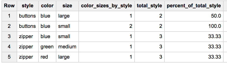
As an example, let’s use a CTE to throw some fake data into BigQuery and ask for a breakdown of counts by color and style, a total of items by style, and the percentage of any given color-style-size combo to the total number of items in that style.

With a window function, you can ask for all of those breakdowns in a single query:

WITH
  inventory AS (
  SELECT 'buttons' AS style, 'blue' AS color, 'large' AS size
  UNION ALL SELECT 'buttons', 'blue', 'small'
  UNION ALL SELECT 'buttons', 'blue', 'small'
  UNION ALL SELECT 'zipper', 'red', 'large'
  UNION ALL SELECT 'zipper', 'blue', 'small'
  UNION ALL SELECT 'zipper', 'green', 'medium')
SELECT
  style,
  color,
  size,
  COUNT(1) AS color_sizes_by_style,
  COUNT(style) OVER(PARTITION BY style) as total_style,
  ROUND(COUNT(1) * 100 / COUNT(style) OVER(PARTITION BY style),2) AS percent_of_total_style
FROM
  inventory
GROUP BY 1, 2, 3
ORDER BY 1, 2, 3

In your result set you get the expected count by style, color, and size for each group of items, but now, because of the window function, you’ve also been able to do a calculation for each row that uses a different grouping – in this case a less granular, style-only grouping – to get a total count from a different set of rows.

The window you get with the OVER() function let’s you define your input distinctly from the way you’ve defined it in your main query, but then returns a value for each row into the query. Previously, I would have done this with a sub-select or some post-processing, but now I understand how to do computation over multiple data breakdowns as part of a normal query.

I’m sure the name “window function” has some other origin, but I like to think of it as giving you a window into other rows in the table that you can reach through and steal data from.

Check out these BigQuery docs on Analytic Functions for deeper explanation and some cool examples.

Aggregates are Lies

Finally, I want to encourage you to be skeptical of aggregate data for two big reasons. First, aggregates are lies – real, interesting, and accurate data is hidden inside the fluctuations you roll up into your aggregate data. Don’t be fooled.

Second, as you learn to write more complicated queries, you’ll be tempted to use your fancy tools right away. Don’t do it.

Any time you’re tackling a new query with new data, you should pour over the undisturbed rows to get a feel for what kinds of variations are hidden there.

I don’t have formal rules yet for developing complicate analytics queries, but if I had to put what I think the process looks like into an ordered list today, I would do something like this:

1. Preview complete rows of the data, not just columns you want to roll up.
2. Do some simple ordering on column values to see ranges and outliers.
3. Do some simple grouping with counts on potentially useful columns to see breakdowns of data.
4. If possible, validate calculations side-by-side with raw data, at least for a sanity check.

Aggregate data tells a lot of important stories, I’m not denying that. But you’re in an interesting position as a software engineer who can write more analytical SQL. You get to see the resulting data AND the code that generated it.

Go slow with the data and piece together the specifics as much as possible. That will tell you a lot more about how your code is interacting with the world than looking at rolled-up, averaged, grouped, or otherwised calculated numbers.