When you are reporting on metrics over time, sometimes your data will have missing entries on certain days.

In these cases, it’s useful to be able to ensure that every date shows up in your report, regardless of whether or not there is a metric in the dataset for that date.

Let’s use daily user logins to a website for a reporting metric to illustrate how you solve this problem.

Quick clarification before we dive into the example: I’m writing this as a throwaway query on Redshift, but if you’re using Postgres there are some sweet shortcuts that make some of the steps below even easier. If you’re using something outside of those two database systems, I hope at least the strategies are clear.

Group By Date + Sum

Our first cut at the data uses a simple GROUP BY and SUM to show the counts per day of user logins:

SELECT
date,
SUM(count) as count
FROM (
  SELECT date, count FROM (SELECT '2019-09-01', 115) as r(date, count)
  UNION ALL
  SELECT date, count FROM (SELECT '2019-09-02', 98) as r2(date,count)
  UNION ALL
  SELECT date, count FROM (SELECT '2019-09-04', 451) as r4(date, count)
  UNION ALL
  SELECT date, count FROM (SELECT '2019-09-05', 239) as r5(date, count)
  UNION ALL
  SELECT date, count FROM (SELECT '2019-09-06', 75) as r6(date, count)
  UNION ALL
  SELECT date, count FROM (SELECT '2019-09-07', 306) as r7(date, count)
)
GROUP BY date

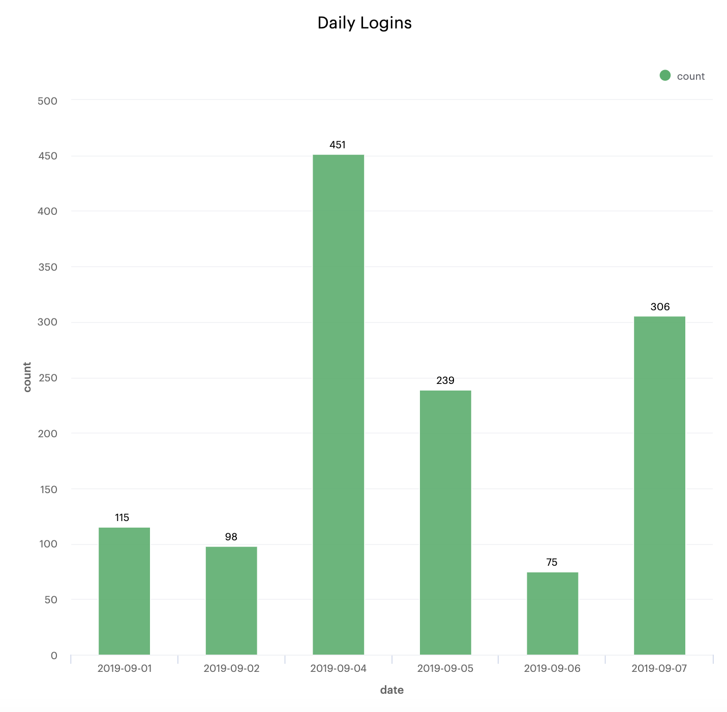
You might see the problem in the sample data in the SQL statement already, but if you look at the dates on the x-axis of the graph, you’ll notice that there’s no entry for 9/3/2019. According to the data, there were no logins that day. And while that might be true, that’s not the best way to report on daily user logins.

What To Do About Zero?

Remember, our goal is to return a full series of dates and login counts for all the days in the report range.

There are alternatives to solving this problem directly in SQL.

You could:

• fill in the gaps after you get your query results back and before you build the report (a strategy you’ll see in a lot of web applications)
• ensure that every day has a zero entry in the database for every metric (don’t do this)

Here, we are going to dynamically fill in the gaps using SQL.

Filling in the Gaps

The key concept you need to keep in mind to fill in the gaps is this: since your table doesn’t have an entry for every date, you need to join on another table that does.

There are 3 ways to get your full date range table:

1. Create a “numbers table” in your database with all the possible dates you’ll ever need
2. Use a function that generates the date range for you (see generate_series in Postgres)
3. Generate the range as part of your query by counting rows in another table that is big enough to cover the range you need

If that third option sounds like a mouthful, good. Keep reading. That’s the one we’re going to unpack.

Here’s what the “full date range” query looks like:

WITH dates AS (
  SELECT
    '2019-09-10'::date - ROW_NUMBER() OVER() as date
  FROM
    some_big_enough_table
  LIMIT 14
), logins AS (
  SELECT date, count FROM (SELECT '2019-09-01'::date, 115) as r(date, count)
  UNION ALL
  SELECT date, count FROM (SELECT '2019-09-02'::date, 98) as r2(date,count)
  UNION ALL
  SELECT date, count FROM (SELECT '2019-09-04'::date, 451) as r4(date, count)
  UNION ALL
  SELECT date, count FROM (SELECT '2019-09-05'::date, 239) as r5(date, count)
  UNION ALL
  SELECT date, count FROM (SELECT '2019-09-06'::date, 75) as r6(date, count)
  UNION ALL
  SELECT date, count FROM (SELECT '2019-09-07'::date, 306) as r7(date, count)
)
SELECT
TO_CHAR(dates.date, 'MM/DD/YYYY') as date,
COALESCE(logins.count,0) as count
FROM
dates
LEFT OUTER JOIN
logins
ON dates.date = logins.date
WHERE
dates.date >= '2019-09-01' and dates.date <= '2019-09-07'
ORDER BY dates.date

Let’s break down what’s going on from top to bottom:

The WITH clause is a Common Table Expression (CTE), that is basically a reusable piece of SQL that gets executed before your main SELECT. I like it for readability, especially compared to nested subqueries.

Inside the CTE, we’re generating our date range, which we will uses as the left side of our LEFT OUTER JOIN. This is the key to having all possible dates represented in our final result.

We are generating dates by subtracting an integer from the hardcoded date at the end of the range we want: '2019-09-10'::date - ROW_NUMBER() OVER() as date. Hardcoding in this case is mostly to make the example easier to read.

The integer we are subtracting comes from the ROW_NUMBER window function. It’s important to convince yourself that the pieces of your complicated SQL queries are actually doing what you think they are doing, so try it out:

SELECT
  ROW_NUMBER() OVER()
FROM 
  some_big_enough_table
LIMIT 10;

Should give you back this:

 row_number 
------------
          1
          2
          3
          4
          5
          6
          7
          8
          9
         10
(10 rows)

some_big_enough_table is any table in your database that has enough rows to generate the date range you want in the query. ROW_NUMBER is just counting the rows for you. It’s a hack to get a series of numbers in play. In Redshift, where “set returning functions” aren’t supported, we use this any time we need a large ordered set of integers to work with.

In this case, we can combine the integers with a hardcoded date, do a little date math, and get the range we want:

        date         
---------------------
 2019-09-09 00:00:00
 2019-09-08 00:00:00
 2019-09-07 00:00:00
 2019-09-06 00:00:00
 2019-09-05 00:00:00
 2019-09-04 00:00:00
 2019-09-03 00:00:00
 2019-09-02 00:00:00
 2019-09-01 00:00:00
 2019-08-31 00:00:00
 2019-08-30 00:00:00
 2019-08-29 00:00:00
 2019-08-28 00:00:00
 2019-08-27 00:00:00
(14 rows)

Now that we have a complete date range, we can join on it as a reference table. With the LEFT OUTER JOIN, we’re taking everything from the date range table, and knitting in the rows from our metrics table by joining on date.

COALESCE, another one of my favorite functions, is doing the work of filling in the missing zero:

    date    | count 
------------+-------
 09/01/2019 |   115
 09/02/2019 |    98
 09/03/2019 |     0
 09/04/2019 |   451
 09/05/2019 |   239
 09/06/2019 |    75
 09/07/2019 |   306
(7 rows)

Without the COALESCE(logins.count,0) as count, we would still have all our dates, but in the second column we would have a NULL value for 9/3/2019:

    date    | count 
------------+-------
 09/01/2019 |   115
 09/02/2019 |    98
 09/03/2019 |      
 09/04/2019 |   451
 09/05/2019 |   239
 09/06/2019 |    75
 09/07/2019 |   306
(7 rows)

COALESCE basically says, “give me logins.count but if you don’t have it, I’ll take a 0”.

Most importantly, we now can build a chart that has one entry per day, whether or not there is a corresponding metric value:

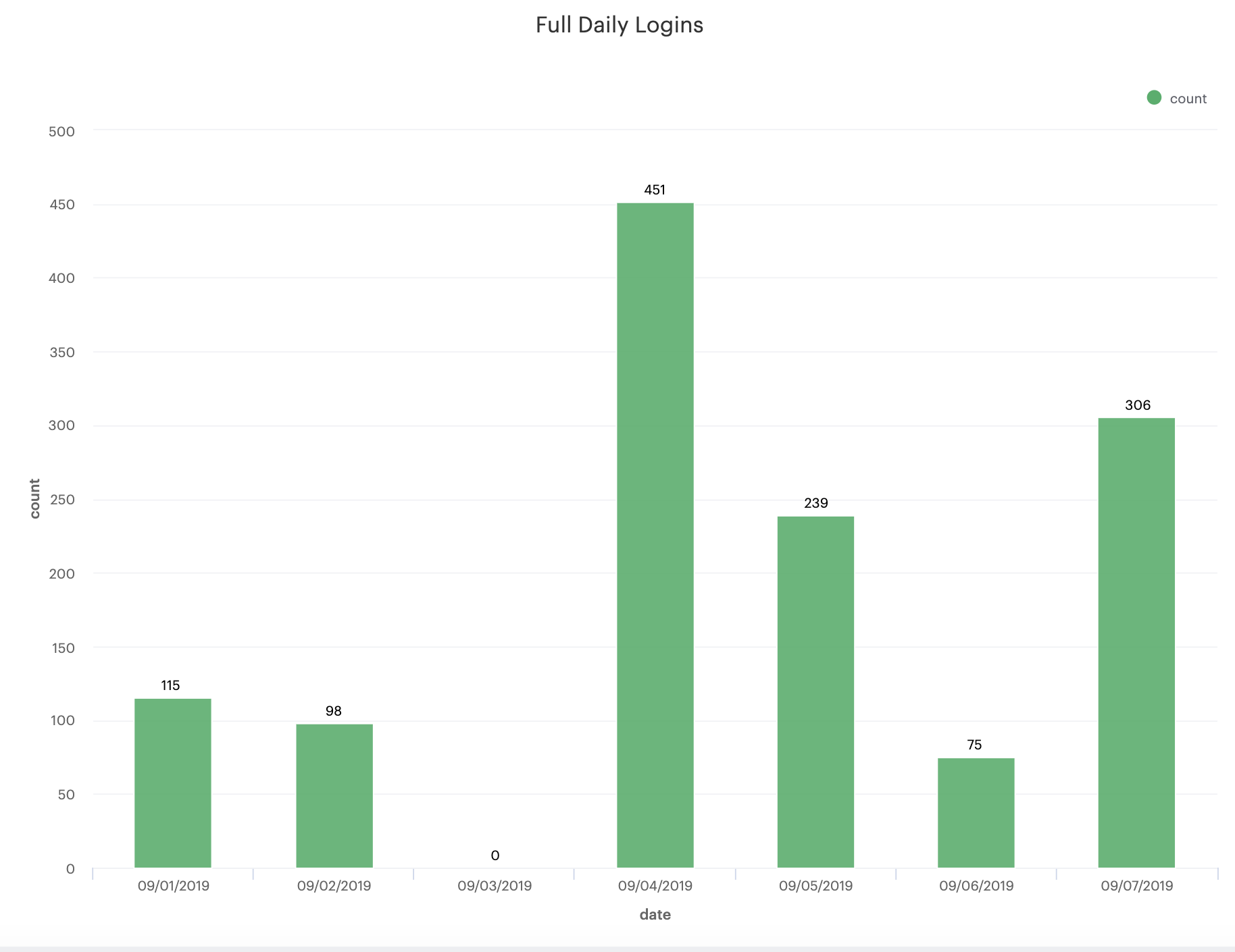
Again, the specific functions and implementations are going to vary depending on the type of database system you’re using, but hopefully the underlying SQL concept is clear and you have some strategies for generating baseline structure and data for your SQL reporting.