In this tip, we want to look at a concise way to shows changes in your data.

I tend to think of this type of problem as a going from “finding” data to “describing” data. For example, if you know how to get every value for a user in the database for the last 30 days, then you can “find” data. When you calculate aggregates of that data using functions like MAX, MIN, SUM, or AVG, you are now “describing” the data.

In this post we’re going to introduce describing the data by showing how one value changes over time. In other words, you’ll be able to answer questions like how much did today’s value change from yesterday’s?

Get a Baseline Using Aggregates

We’ll start with a table called daily_metrics. There is a create script here if you want to follow along in your own database.

First, we’ll do an orientation query to see what’s in the table:

SELECT
  metric,
  MIN(date) as first_metric,
  MAX(date) as last_metric,
  ROUND(AVG(count),2) as avg_value,
  COUNT(metric) as total_entries
FROM daily_metrics
GROUP BY metric
ORDER BY metric;

Which gives us back:

 metric | first_metric | last_metric | avg_value | total_entries 
--------+--------------+-------------+-----------+---------------
 A      | 2019-09-01   | 2019-09-07  |    221.71 |             7
 B      | 2019-09-01   | 2019-09-07  |    149.71 |             7
(2 rows)

As I’ve written before, writing complicated SQL is really about layering information. At each step in the query-writing process, you want to convince yourself that the data you are returning is still correct.

Now that we know our table contains multiple metrics, we can focus in on a single metric to make the query writing process easier.

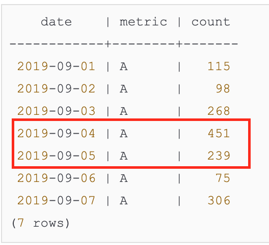
Let’s zoom in on Metric A:

SELECT
  *
FROM daily_metrics
WHERE metric = 'A'
ORDER BY date;

    date    | metric | count 
------------+--------+-------
 2019-09-01 | A      |   115
 2019-09-02 | A      |    98
 2019-09-03 | A      |   268
 2019-09-04 | A      |   451
 2019-09-05 | A      |   239
 2019-09-06 | A      |    75
 2019-09-07 | A      |   306
(7 rows)

For day-over-day change, you can see that some days the count goes up and some days it goes down. At this point, you might export the data and manipulate it in a spreadsheet, but SQL does give you the tools to work with the changing values directly.

If we want to capture change between values, we need the right mental model for the table and row structure we’re working with, relative to the functions we’ll use to calculate over the row values.

In SQL, this is a “window”. If you are used to thinking of query results as a table made up of rows, then a window over that table is a particular sub-set of those rows and values.

Have you ever made a rectangle with the thumbs and index fingers on both of your hands, squinted, and looked around the room through that rectangle? That’s kind of what SQL window functions are doing to your data.

I highly recommend this post if you want to go deeper on window functions.

Find Previous Row Values with LAG

To get a feel for how a window function works, we’ll use LAG. As you can probably guess, LAG looks “back” a row in your data and grabs the column value you specify.

So this:

SELECT
  date,
  metric,
  count,
  LAG(count) OVER() as previous_count
FROM daily_metrics
WHERE metric = 'A'
ORDER BY date;

The query above should return the previous count for each row. Does it?

    date    | metric | count | previous_count 
------------+--------+-------+----------------
 2019-09-01 | A      |   115 |             75
 2019-09-02 | A      |    98 |               
 2019-09-03 | A      |   268 |            451
 2019-09-04 | A      |   451 |            239
 2019-09-05 | A      |   239 |             98
 2019-09-06 | A      |    75 |            268
 2019-09-07 | A      |   306 |            115
(7 rows)

Maybe? LAG might have done what I said it was going to do, but from the way we ran the experiment, it’s kind of hard to tell.

There’s one crucial missing piece on the query above: OVER(). SQL gives us a ton of control over how to define the window and it happens in the OVER() clause. We didn’t define it at all, so we basically said “give us the previous count” without out specifying previous to what.

Let’s try ordering by date inside the OVER clause (we’ll also order the final results by date for readability):

SELECT
  date,
  metric,
  count,
  LAG(count) OVER(ORDER BY date) as previous_count
FROM daily_metrics
WHERE metric = 'A'
ORDER BY date

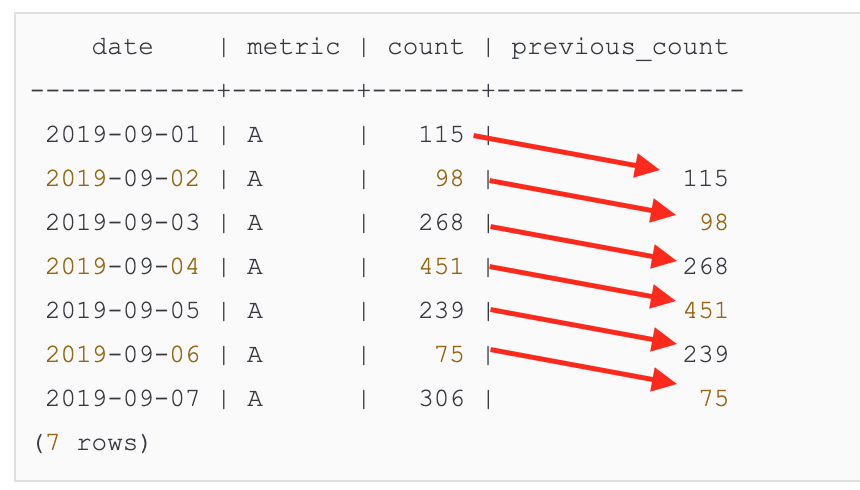
Now we have:

    date    | metric | count | previous_count 
------------+--------+-------+----------------
 2019-09-01 | A      |   115 |               
 2019-09-02 | A      |    98 |            115
 2019-09-03 | A      |   268 |             98
 2019-09-04 | A      |   451 |            268
 2019-09-05 | A      |   239 |            451
 2019-09-06 | A      |    75 |            239
 2019-09-07 | A      |   306 |             75
(7 rows)

Where almost every row has it’s previous count column value in the previous_count column:

I don’t know you if you’re convinced, but that’s about as far as I usually go to convince myself I know how a piece of my query works. Now I’m confident that we can start calculating changes in values.

Calculate Change

Let’s do a simple “current minus previous” operation to express change day-over day:

SELECT
  date,
  metric,
  count,
  LAG(count) OVER(ORDER BY date) as previous_count,
  count - LAG(count) OVER(ORDER BY date) as change
FROM daily_metrics as mc
WHERE metric = 'A'
ORDER BY date

Instead of just showing the change, I like to keep count and previous count around for reference, to check that the math actually works:

    date    | metric | count | previous_count | change 
------------+--------+-------+----------------+--------
 2019-09-01 | A      |   115 |                |       
 2019-09-02 | A      |    98 |            115 |    -17
 2019-09-03 | A      |   268 |             98 |    170
 2019-09-04 | A      |   451 |            268 |    183
 2019-09-05 | A      |   239 |            451 |   -212
 2019-09-06 | A      |    75 |            239 |   -164
 2019-09-07 | A      |   306 |             75 |    231
(7 rows)

Extend to All Metrics

At this point, feeling confident, we can remove our filter on Metric A and it should just work for all metrics, right???

SELECT
  date,
  metric,
  count,
  LAG(count) OVER(ORDER BY date) as previous_count,
  count - LAG(count) OVER(ORDER BY date) as change
FROM daily_metrics as mc
ORDER BY date

Uh oh, mixing metrics gives us mess of rows and we can’t easily tell which row is treated as previous, just based on date order. Our calculations look off!

    date    | metric | count | previous_count | change 
------------+--------+-------+----------------+--------
 2019-09-01 | A      |   115 |             38 |     77
 2019-09-01 | B      |    38 |                |       
 2019-09-02 | A      |    98 |             14 |     84
 2019-09-02 | B      |    14 |            115 |   -101
 2019-09-03 | B      |    77 |            268 |   -191
 2019-09-03 | A      |   268 |             98 |    170
 2019-09-04 | B      |   203 |            451 |   -248
 2019-09-04 | A      |   451 |             77 |    374
 2019-09-05 | B      |   251 |            239 |     12
 2019-09-05 | A      |   239 |            203 |     36
 2019-09-06 | B      |   300 |             75 |    225
 2019-09-06 | A      |    75 |            251 |   -176
 2019-09-07 | A      |   306 |            165 |    141
 2019-09-07 | B      |   165 |            300 |   -135
(14 rows)

What if we order by metric and date inside the window?

SELECT
  date,
  metric,
  count,
  LAG(count) OVER(ORDER BY metric, date) as previous_count,
  count - LAG(count) OVER(ORDER BY metric, date) as change
FROM daily_metrics as mc
ORDER BY metric, date

Almost! There’s one problem row in the results below:

    date    | metric | count | previous_count | change 
------------+--------+-------+----------------+--------
 2019-09-01 | A      |   115 |                |       
 2019-09-02 | A      |    98 |            115 |    -17
 2019-09-03 | A      |   268 |             98 |    170
 2019-09-04 | A      |   451 |            268 |    183
 2019-09-05 | A      |   239 |            451 |   -212
 2019-09-06 | A      |    75 |            239 |   -164
 2019-09-07 | A      |   306 |             75 |    231
 2019-09-01 | B      |    38 |            306 |   -268
 2019-09-02 | B      |    14 |             38 |    -24
 2019-09-03 | B      |    77 |             14 |     63
 2019-09-04 | B      |   203 |             77 |    126
 2019-09-05 | B      |   251 |            203 |     48
 2019-09-06 | B      |   300 |            251 |     49
 2019-09-07 | B      |   165 |            300 |   -135
(14 rows)

Can you spot it? We sorted by metric, then date in our lag function and did the same in the final results, so you have a date-ordered set of Metric A, then a date-ordered set of Metric B, but look at the first Metric B row:

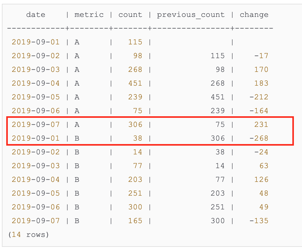
The first Metric B row has a previous count that was the last Metric A row. That’s not accurate, is it? The 9/7/2019 value for Metric A does not precede the 9/1/2019 value for Metric B, but if we rely on order alone, that’s how the data gets calculated.

Fortunately there is another element of a window function that gives us full control of our subsets of data: PARTITION BY.

Define a Partition for More Control over Grouping

SELECT
  date,
  metric,
  count,
  LAG(count) OVER(PARTITION BY metric ORDER BY date) as previous_count,
  count - LAG(count) OVER(PARTITION BY metric ORDER BY date) as change
FROM daily_metrics as mc
ORDER BY metric, date

Now the first Metric B has a null previous count, just like the first row of Metric A:

    date    | metric | count | previous_count | change 
------------+--------+-------+----------------+--------
 2019-09-01 | A      |   115 |                |       
 2019-09-02 | A      |    98 |            115 |    -17
 2019-09-03 | A      |   268 |             98 |    170
 2019-09-04 | A      |   451 |            268 |    183
 2019-09-05 | A      |   239 |            451 |   -212
 2019-09-06 | A      |    75 |            239 |   -164
 2019-09-07 | A      |   306 |             75 |    231
 2019-09-01 | B      |    38 |                |       
 2019-09-02 | B      |    14 |             38 |    -24
 2019-09-03 | B      |    77 |             14 |     63
 2019-09-04 | B      |   203 |             77 |    126
 2019-09-05 | B      |   251 |            203 |     48
 2019-09-06 | B      |   300 |            251 |     49
 2019-09-07 | B      |   165 |            300 |   -135
(14 rows)

The lag function gets applied to each partition, which we’ve been able to define here - kind of like a GROUP BY metric expression without actually doing the GROUP BY – independently of the other partition or groups of rows.

Do More with Windows

While the LAG function and its opposite LEAD are kind of special cases, you can extend this idea to a lot of other functions that are useful for group-isolated calculations.

Any time you are trying to describe something about an individual row along with something about the group that row belongs to, use a window function.

For example:

• Each student’s latest test score and their average for the year
• Every athlete’s height next to the height of the tallest player on each team
• The last time you spotted each bird species in your bird watching journal next to an entry for each bird

For a more window function fun, check out these exercises from Julia Evans.