Whenever you have two sets of data and you need to find the entries that are in your first set, but not in your second set, use this pattern.

Let’s say you have an application that tracks user sign-ups separately for user sign-ins. You might be interested in knowing which users have signed up, but never signed in.

Postgres makes it easy to mock up some sample data so we can work through this use case.

First, create a series of sign-ups:

CREATE TABLE sign_ups AS (
    SELECT 'User ' || generate_series(1,5) as username, '2019-01-01' as date
);

postgres=# SELECT *  FROM sign_ups;
 username |    date    
----------+------------
 User 1   | 2019-01-01
 User 2   | 2019-01-01
 User 3   | 2019-01-01
 User 4   | 2019-01-01
 User 5   | 2019-01-01
(5 rows)

I stole that string concatenation techique from this post which has some other cool data generation ideas in it too.

Now we’ll do a series of sign-ins over the subsequent days, but only for users 1,2, and 3.

CREATE TABLE sign_ins AS (
  SELECT *
  FROM (
    SELECT generate_series('2019-01-02', '2019-01-04', '1 day'::interval) as date
  ) d 
  CROSS JOIN
  (
    SELECT 'User ' || generate_series(1,3) as username
  ) m
);

SELECT username, date FROM sign_ins ORDER BY username, date;

 username |          date          
----------+------------------------
 User 1   | 2019-01-02 00:00:00-05
 User 1   | 2019-01-03 00:00:00-05
 User 1   | 2019-01-04 00:00:00-05
 User 2   | 2019-01-02 00:00:00-05
 User 2   | 2019-01-03 00:00:00-05
 User 2   | 2019-01-04 00:00:00-05
 User 3   | 2019-01-02 00:00:00-05
 User 3   | 2019-01-03 00:00:00-05
 User 3   | 2019-01-04 00:00:00-05
(9 rows)

We know our result should be that users 4 and 5 never signed in.

Give Me Everything EXCEPT…

There is a way to write this query that almost looks exactly how you’d phrase it in plain English, “Give me everything from table 1, except what’s in table 2”:

SELECT username FROM sign_ups
EXCEPT
SELECT username FROM sign_ins GROUP BY username;

 username 
----------
 User 5
 User 4
(2 rows)

In this case, the EXCEPT query is pretty readable, and with our sample data, pretty fast.

But there is an alternate way to solve this problem that will be powerful to know and often more performant.

Anti Join Your Tables

The second way to get the missing data combines a LEFT OUTER JOIN and a WHERE clause into something called an “Anti Join.”

We use the LEFT OUTER JOIN on our sign-ups table – which means we want to potentially include all rows from the sign-ups table, but then we do something tricky with the WHERE clause:

SELECT
  su.username
FROM
  (
    SELECT username FROM sign_ups
  ) su
LEFT OUTER JOIN
  (
    SELECT username FROM sign_ins GROUP BY username
  ) si
ON
  su.username = si.username
WHERE
  si.username IS NULL;

 username 
----------
 User 4
 User 5
(2 rows)

Here we’re saying WHERE si.username IS NULL which means we are asking for anything in the sign-ups table that does not have a matching row in the sign-ins table.

Our final result is the same, but it will be easier to visualize what is going on if we project the full set of values from both tables, before the special WHERE filter is applied.

Running the previous query without the filter, just a regular LEFT OUTER JOIN:

SELECT
  su.username as sign_up_username,
  si.username as sign_in_username
FROM
  (
    SELECT username FROM sign_ups
  ) su
LEFT OUTER JOIN
  (
    SELECT username FROM sign_ins GROUP BY username
  ) si
ON
  su.username = si.username

You can see more clearly where the missing data is now:

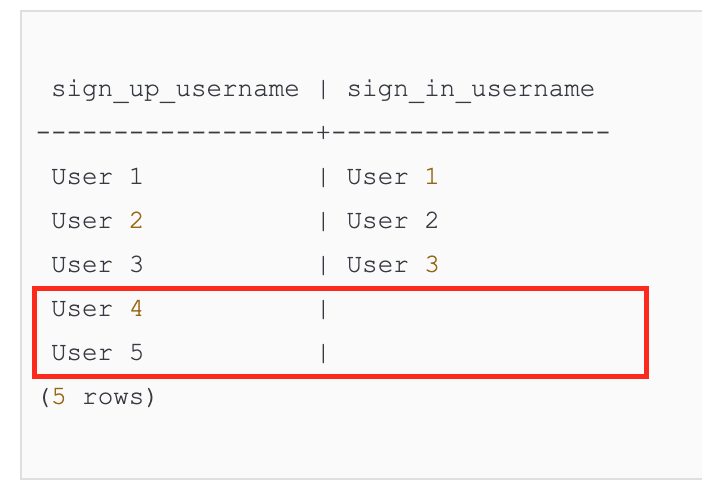
We have 5 users who have signed up, but only 3 who have signed in, meaning 3 rows from the sign-ins table will have username values and 2 rows from the sign-ins table, which show up here in the sign_in_username column, will have null values.

When we go back and add WHERE si.username IS NULL to our LEFT OUTER JOIN, we are explictly asking for just the null rows.

Which Query is Better?

SQL is considered a “declarative” programming language, which basically means you tell the query engine what you want and you don’t care how it gets it for you. Most of the time this is a fine arrangement.

However, if you have two different queries and you really want to know whether the query engine will treat them differently, in Postgres you can just ask. You can see the query plan by running EXPLAIN ANALYZE.

Initially, I picked the example data for this post to be readable, so it was easy to reason about missing rows. I didn’t think there was any performace difference between the two solutions.

But then I tried the queries on larger tables:

CREATE TABLE sign_ups_big AS (
    SELECT 'User ' || generate_series(1,100000) as username, '2019-01-01' as date
);

CREATE TABLE sign_ins_big AS (
  SELECT *
  FROM (
    SELECT generate_series('2019-01-02', '2019-01-04', '1 day'::interval) as date
  ) d 
  CROSS JOIN
  (
    SELECT 'User ' || generate_series(1,900) as username
  ) m
);

Was there a difference with 2,700 sign-ins against 100,000 sign-ups? Yes!

Here is the query plan for the EXCEPT version:

EXPLAIN ANALYZE SELECT username FROM sign_ups_big
EXCEPT
SELECT username FROM sign_ins_big GROUP BY username

                                                                 QUERY PLAN                                                                  
---------------------------------------------------------------------------------------------------------------------------------------------
 SetOp Except  (cost=13853.33..14357.83 rows=100000 width=36) (actual time=2315.169..2380.763 rows=99100 loops=1)
   ->  Sort  (cost=13853.33..14105.58 rows=100900 width=36) (actual time=2315.156..2360.786 rows=100900 loops=1)
         Sort Key: "*SELECT* 1".username
         Sort Method: external merge  Disk: 2576kB
         ->  Append  (cost=0.00..2705.75 rows=100900 width=36) (actual time=0.010..38.108 rows=100900 loops=1)
               ->  Subquery Scan on "*SELECT* 1"  (cost=0.00..2637.00 rows=100000 width=14) (actual time=0.010..26.048 rows=100000 loops=1)
                     ->  Seq Scan on sign_ups_big  (cost=0.00..1637.00 rows=100000 width=10) (actual time=0.009..12.738 rows=100000 loops=1)
               ->  Subquery Scan on "*SELECT* 2"  (cost=50.75..68.75 rows=900 width=12) (actual time=0.797..1.082 rows=900 loops=1)
                     ->  HashAggregate  (cost=50.75..59.75 rows=900 width=8) (actual time=0.797..0.948 rows=900 loops=1)
                           Group Key: sign_ins_big.username
                           ->  Seq Scan on sign_ins_big  (cost=0.00..44.00 rows=2700 width=8) (actual time=0.008..0.237 rows=2700 loops=1)
 Planning time: 0.162 ms
 Execution time: 2389.068 ms
(13 rows)

Compared to the LEFT OUTER JOIN:

EXPLAIN ANALYZE SELECT
  su.username
FROM
  (
    SELECT username FROM sign_ups_big
  ) su
LEFT OUTER JOIN
  (
    SELECT username FROM sign_ins_big GROUP BY username
  ) si
ON
  su.username = si.username
WHERE
  si.username IS NULL;
  
                                                          QUERY PLAN                                                           
-------------------------------------------------------------------------------------------------------------------------------
 Hash Anti Join  (cost=80.00..8098.25 rows=50000 width=10) (actual time=1.431..28.122 rows=99100 loops=1)
   Hash Cond: (sign_ups_big.username = sign_ins_big.username)
   ->  Seq Scan on sign_ups_big  (cost=0.00..1637.00 rows=100000 width=10) (actual time=0.007..9.029 rows=100000 loops=1)
   ->  Hash  (cost=68.75..68.75 rows=900 width=8) (actual time=1.157..1.157 rows=900 loops=1)
         Buckets: 1024  Batches: 1  Memory Usage: 44kB
         ->  HashAggregate  (cost=50.75..59.75 rows=900 width=8) (actual time=0.865..0.992 rows=900 loops=1)
               Group Key: sign_ins_big.username
               ->  Seq Scan on sign_ins_big  (cost=0.00..44.00 rows=2700 width=8) (actual time=0.005..0.255 rows=2700 loops=1)
 Planning time: 0.088 ms
 Execution time: 33.975 ms
(10 rows)

Execution time: 2389.068 ms for the EXCEPT query vs. Execution time: 33.975 ms for the Anti Join.

Now, reading query plans is an art unto itself and I refer you to depesz for further reading if you really want to go deep.

All you need to know right now is that query plans make sense when you read them from the bottom up and from the most indented to the least. What you see on the first line is the last thing to happen, but it’s what the planner is driving towards, so it’s useful to call it out right away.

In our two examples, we’re ultimately solving the problem with a SetOp Except in the EXCEPT query and Hash Anti Join in the LEFT OUTER JOIN query.

You can see the steps we will take to get to the SetOp Except, by reading through the arrows in the query plan. Remember they get executed bottom to top, so we are going to:

• Scan each table from the subqueries (grouping the data from the sign-ins table by username)
• Append the rows from the scans to one big list
• Sort everything in the big list
• Perform the except operation

It turns out, building a sorted list and removing duplicates is slow when you have as many rows as we now have in the large tables!

But What Does it Cost?

Another way to read the plans that clues you in to performance is to look at the “cost” on each line. Cost here represents “work” for the database engine, not exactly time, but I’ve started to think of all the cost metrics through a relay race analogy. For example, when you see cost=0.00..44.00, the 0 means the runner can start at the beginning of the race, i.e. query execution, and will be running until 44.

As a side note that might ruin the analogy, both sequential scans in both queries start at the same time. Operations can have the same initial cost, i.e. start the race at the same time, whenever they can be performed independent of each other. In the EXCEPT query, the Append operation also starts from 0, since the row data can be appended to our giant yet-to-be-sorted list as soon as we start reading from the tables. Contrast that to the HashAggregate operation that happens above the scan of sign_ins_big. This is the GROUP BY operation, which only happens at 50.75, once all the to-be-grouped data is scanned.

In the LEFT OUTER JOIN query plan, we have Hash Anti Join (cost=80.00..8098.25, which means the final step can’t start until 80 and will run until 8098.25. Compare that to the final step in the EXCEPT query,SetOp Except (cost=13853.33..14357.83. We see a much longer wait time until the last runner can go and a longer run for the last runner – both clues to what we already looked at – adding all the rows together and sorting them to figure out what to exclude is expensive.

Takeaways

It’s tempting to want to draw conclusions about which operations you should always use based on this one example, but I want you to reserve permanent judgement if you can.

Instead, whenever you find yourself with a coin-toss about which query to use, run EXPLAIN ANALYZE and use it as a chance to dig into the underlying mechanics a little more. You will either confirm your intuitions about performance, or find a surprising thread you can pull to go learn something new. That, in my opinion, is the best way to build your skills up over time.

While I think the EXCEPT example here is easy to understand because the query is so straightforward to write, you will find more cases where the Anti Join pattern, or something like it, helps you solve a SQL problem. Get that LEFT OUTER JOIN...WHERE...IS NULL pattern into your muscle memory!